A Look at the heavy left tail and its distribution
Exploring the Expected Shortfall with flexbile distributions
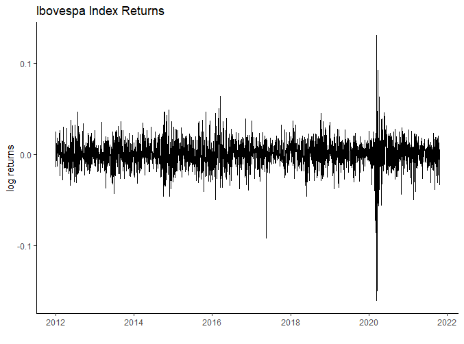
If there is a place where the devil lives, it is in the left tail of the returns distribution.
To further explore what happens in the lower tail, let’s tweak several models to choose one and compare it to a standard distribution.The analysis will be done using the R programming language.
Load Packages and dataset of bovespa Index. You can reproduce this analysis here.
pacman::p_load(tidyverse,ggplot2,dpylr)
readxl::read_excel('bovespa.xlsx') -> bovespa_index
Lets work with logarithmic returns as computed below.
bovespa_index %<>% mutate(returns_log = log(Close/lag(Close))) %>% drop_na()
Below we look for the left tail elements in yellow, here understand that lower tail are values equal to or less than the 5% quantile.
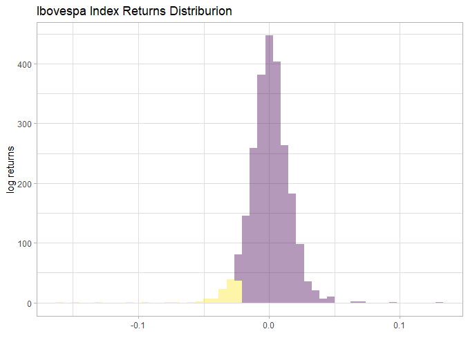
bovespa_index %>% summarise(lower_tail = quantile(probs=c(.05),returns_log)) %>% pull() -> quantile_lower
bovespa_index %<>% mutate(lower_tail = if_else(returns_log <= quantile_lower,1,0))
bovespa_index %>% filter(returns_log <= quantile_lower) -> lower_tail_bovespa
We are using two criteria to select distributions, AIC and BIC.
require(gamlss)
size_sample<- dim(bovespa_index)[1]
fit_dists_aic <- fitDist(lower_tail_bovespa$returns_log,k = 2)
fit_dists_bic <-fitDist(lower_tail_bovespa$returns_log,k = log(size_sample))
GAMLSS are powerful packages for flexible modelling and the package contains many distributions for fit. We use fitDist to find the best fitted model for lower tail data.
fit_dists_aic$fits
fit_dists_bic$fits
| Distribution | AIC | BIC |
|---|---|---|
| Skew t (Azzalini type 2) | -836.7455 | -829.5728 |
A Skew t is a distribution is accounts for heavy tail, and very used in finance ( look 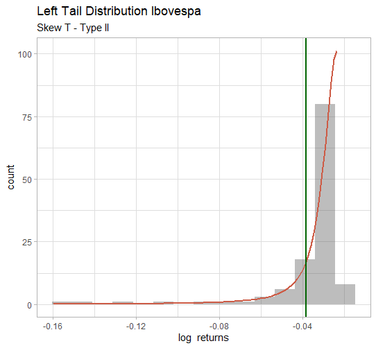 ).
).
The green line is the mean on the lower tail.To calculate it, it was necessary to use the following formula as documented here.
calculate_mean_ST2 <-function(mu,sigma,tau,nu){

  EZ <- ((nu*sqrt(tau))* gamma((tau-1)/2)) /( sqrt(1+nu^2) * sqrt(pi)*gamma(tau/2))
   mean <- mu+sigma*EZ
  return(mean)
}
To compare with the Gaussian distribution we compute the estimated mean and deviation from the lower tail.
min_log_returns<- min(lower_tail_bovespa$returns_log); max_log_returns<- max(lower_tail_bovespa$returns_log);
x_hat <- mean(lower_tail_bovespa$returns_log) #gaussian estimator for \mu
sd_hat <- sd(lower_tail_bovespa$returns_log) # Gaussian estimator for \sigma
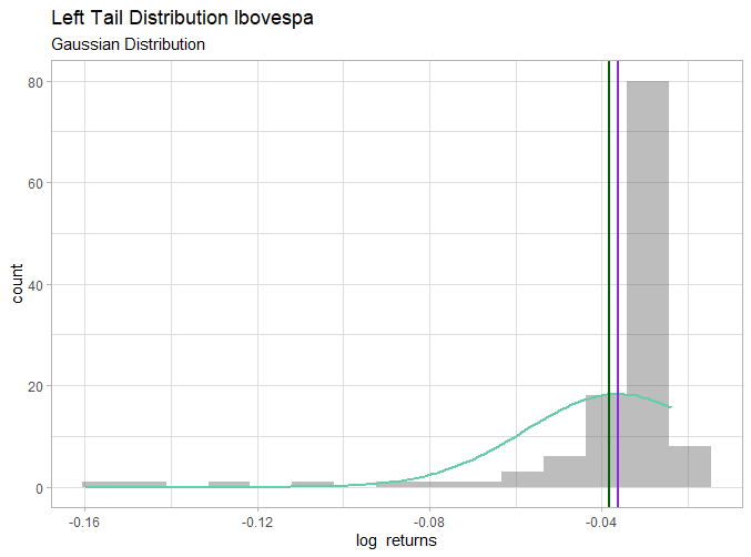
Note that assuming the Gaussian distribution for these data may lead to an overestimation of the mean in the lower tail. The mean for skew-t was -0.038 while for Gaussian it was -0.036.